The distributed and secure nature of blockchain requires independent execution by many decentralized nodes to reach consensus on the next block (see "designing a messaging layer"). Physical limitations constrain a blockchain’s throughput. Not every node can be a supercomputer with 100G networking, and, more importantly, messages can’t be sent between nodes faster than the speed of light. Ultimately, there’s a limit or budget for how much computation can be included in each block. For Ethereum (and Monad), that limit is denominated in gas, an imperfect heuristic of the resource cost by node operators. A user’s transaction is included in a block based on the fee per gas they are willing to pay.
Ethereum’s EIP-1559 introduced the idea of a base fee (a posted price for transaction inclusion). The base fee rises when demand for blockspace is high (block gas used is above target), and falls when demand is low (block gas used is below target). That intuitive feedback loop makes sense for Monad too. However, special consideration is merited when blocks are produced every 400 ms, rather than 12 seconds. There are more opportunities to both gauge recent blockspace demand and update the base fee.
In particular, we designed a new update rule to produce a base fee that is responsive to sustained changes in demand. A twitchy base fee could produce a poor user experience if the base fee spiked dramatically between the time of submission and block proposal. If there’s a sharp increase in the base fee, the user’s transaction would be priced too low and fail to be included for an extended time.
The proposed redesign:
- dampens short-term volatility of the fee;
- responds cautiously when demand is noisy; and
- adjusts decisively when demand shifts persistently.
In this post, we provide an interactive simulation and the intuition for our redesign of the base fee update rule.
Base Fee Simulation
The Update Rule
Monad’s proposed base fee update rule is inspired by practical adaptive methods in optimization, such as RMSprop and Adam. To compute the base fee for the next block, the rule combines three kinds of inputs:
- Measurements from the current block
- $\text{block_gas}_k$ = total gas declared in block $k$. (in the context of Monad, these are the transactions’ gas limits)
- State from past blocks
- Trend: the smoothed average deviation of block gas usage from the target.
- Moment: the smoothed second moment of that deviation.
- Fixed protocol parameters
- $\text{block_gas_limit}$: the maximum gas allowed per block (e.g. 200M).
- $\text{target}$ = target gas usage (set to 80% of the block gas limit).
- $\text{min_base_fee}=100$ MON-gwei: the minimum base fee the system will enforce.
- $\beta=0.96$: smoothing constant for exponential moving averages.
- $\text{max_step_size}=1/28$: caps the maximum per-block adjustment.
- $\varepsilon$: scaling factor, set equal to the target.
Together, the trend and moment describe how consistent or volatile recent demand has been, providing a running estimate of the variance in gas usage relative to the target. This information complements the current block data and protocol parameters, helping the update rule adjust the base fee more cautiously when demand is noisy and more decisively when it is stable.
These inputs are combined in three sequential steps:
1. Update the state
The block’s gas usage is compared against the target. The trend and moment are updated in an exponential smoothing average fashion:
$$\text{trend}_{k+1}=\beta\cdot\text{trend}_k+(1−\beta)(\text{target}−\text{block_gas}_k)$$
$$\text{moment}_{k+1}=\beta\cdot\text{moment}_k+(1−\beta)(\text{target}−\text{block_gas}_k)^2$$
where $\beta=0.96$. This corresponds to a half-life of about 17 blocks, or roughly 7 seconds when blocks are 400 ms. A past block’s influence on the base fee is reduced by half in that time, which means that short-term spikes are quickly faded while sustained trends shape the fee.
Note that using an exponential smoothing average is highly efficient in the amount of required state - only a single scalar is required to represent the sequence of historical values.
2. Compute the learning rate
The effective step size is determined by the following parameters:
$$\eta_k \;=\; \frac{\text{max_step_size} \cdot \varepsilon} {\varepsilon + \sqrt{\text{moment}_{k} - \text{trend}_{k}^2}}$$
- If demand is volatile, the denominator grows, so $\eta_k$ shrinks and updates are gentler. Intuitively, there is less certainty in the required adjustment.
- If demand is stable (low estimated variance of the demand), the denominator is small, so $\eta_k$ approaches the maximum. Intuitively, there is more certainty in the required adjustment.
3. Update the base fee
Finally, the base fee itself is updated according to:
$$\text{base_fee}_{k+1} \;=\;\max\!\Bigg( \text{min_base_fee},\; \text{base_fee}_k \cdot \exp\!\left[ \eta_k \cdot \frac{\text{block_gas}_k - \text{target}} {\text{block_gas_limit} - \text{target}} \right]\Bigg)$$
This exponential form ensures smooth, continuous changes in the base fee. When demand is persistently high or low, the base fee ramps decisively upward or downward until equilibrium is restored. Short-lived demand fluctuations are largely ignored.
Intuition and Behavior Under Different Scenarios
Monad’s base fee update rule is variance-aware. The size of each adjustment depends not only on whether blocks are above or below the target, but also on how consistent demand has been throughout exponentially-smoothed periods of about 17 blocks.
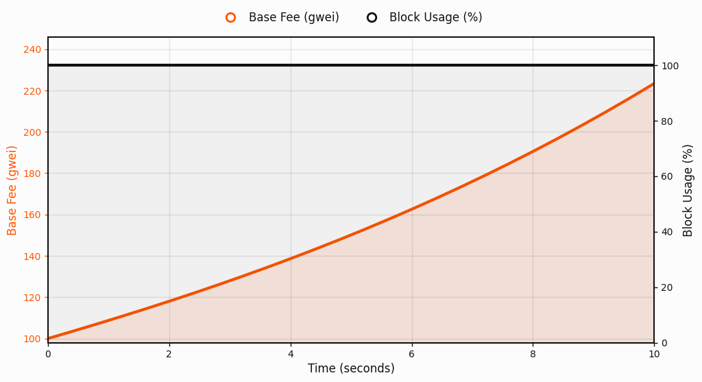
Sustained demand. When blocks are consistently above the target, variance is low, despite the trend being significant. As such, the learning rate $\eta_k$ approaches its maximum, and the base fee ramps decisively upward until equilibrium is restored by rational actors reducing demand as price increases. The same logic applies in the opposite direction when demand is persistently low, leading to a decisive decrease.
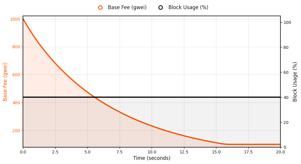
Persistently low demand. Similar to the sustained demand case, variance remains low even though the deviation from the target is significant, but in the opposite direction. In this regime, the learning rate $\eta_k$ also approaches its upper bound, and the base fee decreases decisively until it reaches the minimum level permitted by the protocol. Once at $\text{min_base_fee}$, it remains stable, reflecting an equilibrium under low and steady utilization.
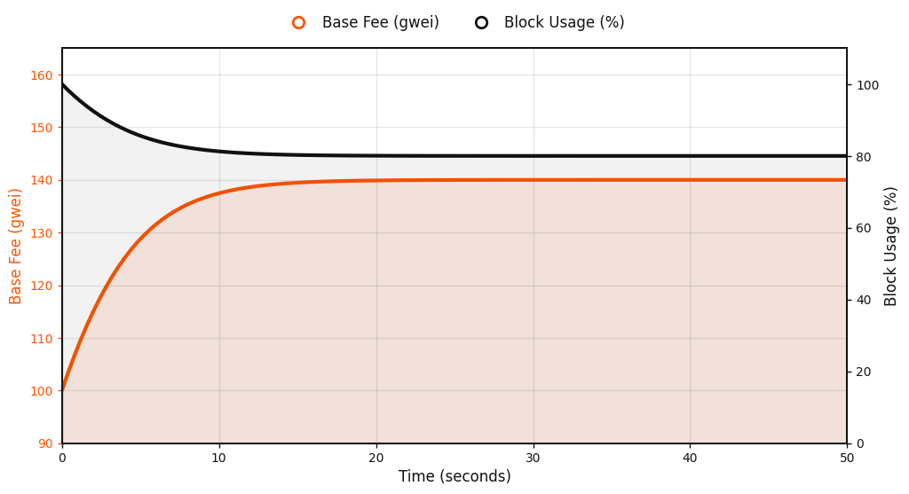
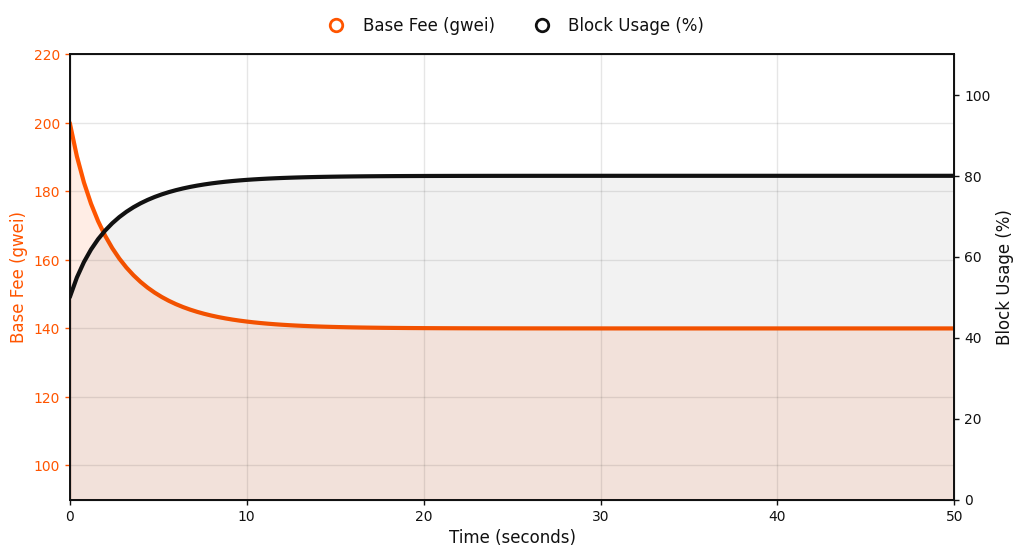
Linear demand response. Imagine that a user's demand for block inclusion is a linear function of price: higher base fees suppress demand, while lower fees encourage it. Then, the equilibrium point occurs where this demand curve crosses the target utilization line, balancing throughput with acceptable cost.

Starting from a base fee below equilibrium, demand exceeds the target. Blocks remain full, and with low variance, the learning rate $\eta_k$ reaches its cap, pushing the base fee upward until it meets the equilibrium point.
Conversely, when starting from a high base fee, block utilization falls below the target. The same adaptive mechanism accelerates downward updates, reducing the fee until usage recovers. In both directions, the feedback loop restores equilibrium quickly and smoothly under linear, rational demand.
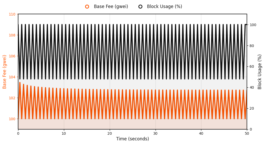
Spiky demand. When blocks alternate between 100% and 60% full, average usage is right at the 80% target, but variance is high. The learning rate $\eta_k$ shrinks, and the base fee responds cautiously. This avoids strong oscillations despite repeated short-lived deviations.
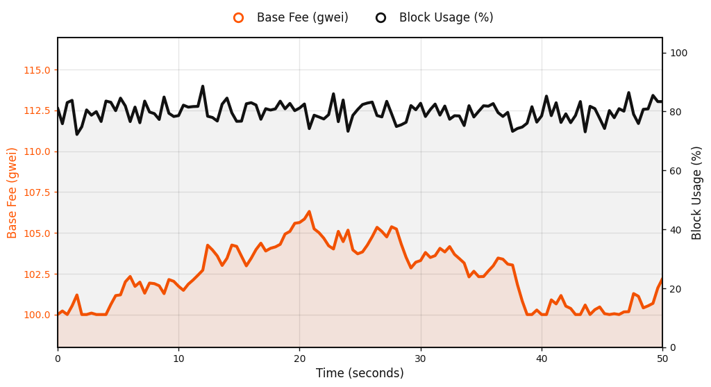
Near target. When gas usage hovers close to the 80% target with only modest noise, the base fee remains stable. Deviations decay with the smoothing half-life ($\beta$=0.96 , about 7 seconds), so transient bursts are quickly faded.
Parameter Choices
The behavior of the base fee update rule is determined by a few protocol parameters. These values control how quickly the fee responds to demand, how long past blocks influence updates, and what level of utilization is targeted.
Minimum base fee = 100 MON-gwei. The minimum base fee is set to 100 MON-gwei. Such a minimum fee covers the nominal costs associated with transaction validation, even when demand is relatively low. It also prevents spam-driven denial-of-service (DoS) attacks, sustaining high gas utilization and throughput. The value is chosen based on user cost considerations: for a simple transfer consuming 21,000 gas, a 100 MON-gwei fee corresponds to approximately 0.002 MON per transaction.
Target utilization = 80%. The block gas target is set to 80% of the block gas limit. This is significantly higher than the 50% target in Ethereum’s EIP-1559, allowing for higher utilization closer to the actual limit of the chain while still leaving room to collect upward demand signals. It’s worth noting that the choice of target affects the magnitude of potential responsiveness. With a target of 0.8, step(3) above can produce an exponentiation term for decreasing the base fee ($\text{block_gas_k = 0}$) that is 4X as large relative to an increase ($\text{block_gas_k = block_gas_limit}$).
Smoothing factor $\beta=0.96$. Trend and moment are updated using exponential smoothing with $\beta=0.96$. This corresponds to a half-life of about 17 blocks, or roughly 7 seconds at 400 ms block times. Short bursts in demand therefore decay quickly, while persistent drifts result in material adjustments.
Maximum step size = 1/28. The learning rate $\eta_k$ is capped so that the per-block adjustment cannot exceed 1/28. This corresponds to an increase of about 3.6% per block, which compounds to roughly a 1.4× increase over 10 blocks (~4 seconds). Note that due to the choice of target, the maximum step size can be multiplied by up to 4 when demand is lower than the target. This extreme case results in a decrease of about 13.3% per block, which compounds to roughly a 76% decrease over 10 blocks (~4 seconds).$\text{*}$
Conclusion
Short spikes are smoothed. Brief bursts of demand have little effect on the base fee, since their influence decays with an approximately 7-second half-life. As a result, the base fee does not overreact to single full blocks, and users are shielded from sharp oscillations in fees; the current base fee is a more stable estimate for future base fees in the near term.
Sustained demand drives the fee. If blocks stay full for many seconds in a row, the base fee reacts quickly, rising until demand no longer exceeds the target. In the extreme, it can reach about 1.4× over 4 seconds. The same responsiveness applies even more quickly in reverse, with the fee declining rapidly when blocks are persistently empty. This asymmetry in responsiveness biases base fees lower, making transactions cheap to include for users.
$\text{*}$ The rate of this adjustment from slower block times is sub-linear due to the more frequent control intervals present over shorter block times (i.e., every block), assuming independence of inter-block demand.
